I would like you to be able to manipulate graphs in 2 and 3 dimensions.
Today we will start with two dimensions.
You should be able to translate and rotate a graph defined parametrically and implicitly.
For polar equations, rotation about the origin by an angle $\phi$ is simply making
the replacement $\theta \rightarrow \theta + \phi$, but translatation is probably easiest
if you change from polar to parametric plot by representing the polar point
$(\theta, r(\theta))$ as a point in rectangular coordinates
$[r(\theta) cos(\theta), r(\theta) sin(\theta)]$ and then plotting the graph
parametrically.
Question #1:
Write a function translate which accepts a pair of expressions in the
parameter t, $x(t)$ and $y(t)$ (representing a parametric curve)
and a point p = [px,py] and the result
is an expression which translates the equation by px in the
$x$-direction and py in the $y$-direction.
Test your function as follows:
> plot( [op(translate([cos(t),sin(t)],[1,-2])), t=0..2*Pi] );
and verify that this is a graph of a circle with origin at $(1,-2)$.
Note that the op is there because plot expects you to give
the parametic equation of the form plot( [xoft, yoft, t=a..b] )
but I would like your function translate to work so that
translate([xoft, yoft], [a, b]) will return [newxoft, newyoft].
Your function should work on any parametric equation that I might give you.
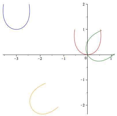
The following equation was rotated $\pi/6$ degrees
clockwise around the point $(2,1)$ and then it was rotated
$\pi/4$ degrees around $(-1,0)$. Find the equation after it
was rotated back.
FYI, I had in this last sentence 'counter clockwise' but I meant 'clockwise'.
This was a mistake that I have since corrected. Your final answer to this question
should be very simple and in this case you will know you have the right answer.
Write a function rotate_origin which takes a parametric equation
$x(t)$ and $y(t)$ (representing a parametric curve)
and an angle $\theta$
and rotates
a point about the origin by an angle $\theta$ (clockwise). Write a function
rotate_point which rotates a parametric curve about a point
by an angle $\theta$ (clockwise). Your function rotate_point should work by
translating your function so that $p$ is at the origin and then rotating by
$\theta$ degrees around the origin and then translating back so that $p$ is
in its original place.
Question #2:
Do the same thing for an implicit equation, that is write a function
translate_implicit, rotate_origin_implict and rotate_point_implicit
so that you can translate and rotate an implicit equation. Test your functions
on the following equations.
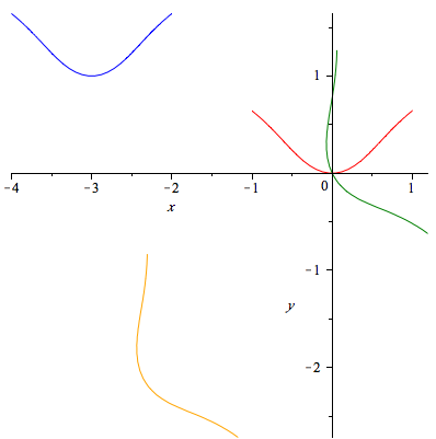
The following equation was rotated $\pi/6$ degrees
clockwise around the point $(2,1)$ and then it was rotated
$\pi/4$ degrees around $(-1,0)$. Find the equation after it
was rotated back.
FYI, I had in this last sentence 'counter clockwise' but I meant 'clockwise'.
This was a mistake that I have since corrected. Your final answer to this question
should be very simple and in this case you will know you have the right answer.
You should open up a new worksheet and start from scratch. You will have to save
your work in a file and upload that file on to the course
moodle. Your
solution should be a sequence of commands where it is easy to change the input
string and after you execute the sequence of commands you should have the
correct output string. Please add documentation to your worksheet to explain how it
works. Just a few sentences is sufficient, but imagine that you were opening up the
worksheet for the first time and wanted to know what it did. You will be marked down
if what you write is not clear and coherent.
You should finish your assignment by Wednesday, November 29 by 11:59pm. Assignments
submitted after this date will be assessed a penalty of 10% per day.